


 18 / 50

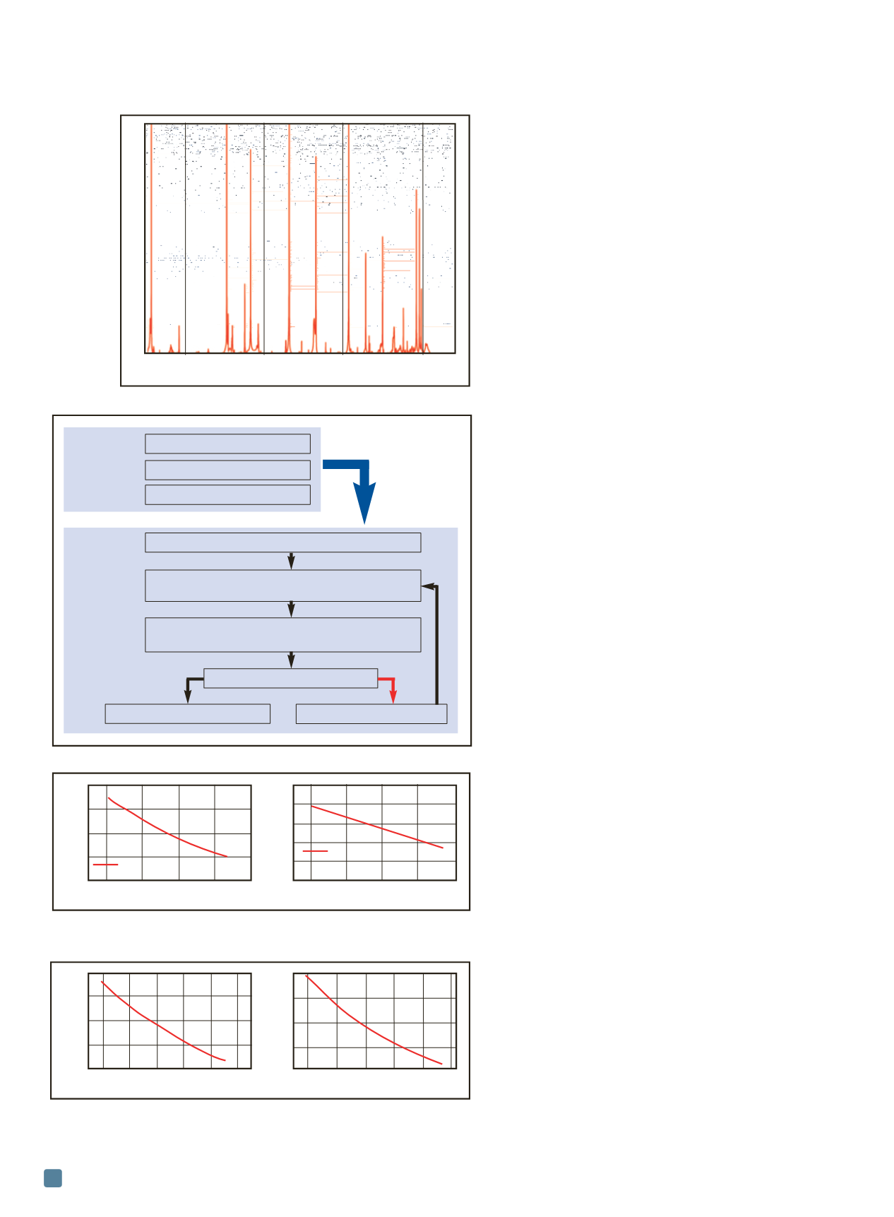
tra are peaks at various frequencies as shown in Fig. 2.
The positions of the peaks correspond to the eigenfre-
quencies of the test sample.
After collecting the resonant frequencies, determining
the elastic constants involves a fairly complicated proce-
dure. Because this is an inverse problem, one must first
provide an initial “guess” regarding the unknown elastic
constants from other means, such as existing knowledge
of similar materials or theoretical modeling. Using these
estimated elastic constants, along with sample geometry
and mass density, the eigenfrequencies of the test sample
can be estimated and compared to the measured data. If
these two sets of frequencies are identical—or the differ-
ence is small enough—then the predicted values can be re-
garded as the sample’s true elastic constants. Otherwise,
the predicted values must be modified and the above steps
repeated. This procedure usually requires a number of it-
erations and is affected by the quality of both the meas-
ured data and initial estimates.
A key step in this data analysis is to find an appropri-
ate algorithm to modify the elastic constants based on dif-
ferences between measured and calculated frequencies.
This is often realized through computer codes and soft-
ware. One common process is the Levenberg-Marquardt
algorithm
[8]
, which is a nonlinear least-squares scheme that
uses Taylor’s expansion to linearize the difference between
measured and calculated frequencies. This data analysis
procedure is illustrated in Fig. 3. RUS theories are ex-
plained further in a textbook by Migliori and Sarrao
[9]
.
Resonant ultrasound spectroscopy
research applications
As previously mentioned, RUS is used to measure the
elastic constants of solid materials in various research areas
including metals, alloys, ceramics, glasses, concretes, and
rocks. Compared to many static testing methods, such as
tensile and bending tests, RUS is nondestructive and can
work with small samples. Compared to other ultrasonic
techniques such as the pulse echo method, RUS features
less preparation and faster sample installation.
Because elastic constants are influenced by other
physical and chemical properties, RUS can be used to ex-
plore many related phenomena, including structural
phase changes, superconducting transitions, magnetic
transitions, and damage accumulation due to micro-
cracking. For example, RUS is used to measure the influ-
ence of porosity on the elastic constants of alumina at
different sintering stages. Young’s modulus as a function
of volume fraction porosity is shown in Fig. 4a
[10]
. This
information can facilitate a deeper understanding of
porosity evolution during sintering and its effect on me-
chanical properties—key aspects in the design and fabri-
cation of engineering ceramics.
Further, RUS measurement can be made under some
extreme conditions such as high and low temperatures.
Figure 4b shows the measurement of Young’s modulus of
a PbTe-based thermoelectric material between room tem-
perature and 673 K (400°C)
[11]
. In this case, Young’s mod-
ADVANCED MATERIALS & PROCESSES •
OCTOBER 2014
18
100
200
300
400
Frequency, kHz
Intensity, a.u.
Fig. 2
—
Sample spectrum obtained from RUS measurement.
Mass density
Geometric parameters
Resonant frequencies
Estimate elastic constants.
Calculate resonant frequencies from mass density,
geometry, and estimated elastic constants.
Determine difference between calculated
frequencies and measured resonant frequencies.
Yes
Is the difference minimized? No
Solution found!
Update elastic constants.
Data
collection
Data
analysis
Fig. 3
—
Schematic of data collection and analysis steps involved in RUS.
Fig. 4
—
RUS is used to determine (a) porosity effect on Young’s modulus
of alumina (after
[10]
), and (b) temperature effect on Young’s modulus of
PbTe-based thermoelectric materials (after
[11]
).
Fig. 5
—
Temperature dependent Young’s modulus as measured by RUS
reveals a diffusion controlled order-disorder phase change: (a) heating/
cooling rate = 5 K/min, (b) heating/cooling rate = 2 K/min
[12]
.
0.05 0.15 0.25 0.35 0.45
Porosity
300 400 500 600 700
Temperature, K
300 400 500 600 700 800
Temperature, K
300 400 500 600 700 800
Temperature, K
Linear trend
60
55
50
45
40
35
52
48
44
40
36
52
48
44
40
36
Young’s modulus, GPa
Young’s modulus, GPa
Young’s modulus, GPa
Young’s modulus, GPa
400
300
200
100
0
Exponential trend
(a) (b)
(a) (b)