


 18 / 74

make poor assumptions such as spherical grain shapes.
However, the increase in 3D microstructural analysis has
led to a number of datasets that can make direct compar-
isons to these models. One example shown in Fig. 1 is the
serial sectioning of a β-titanium alloy, wherein 200 serial
sections spaced 1.5 μm apart were stacked to reconstruct
the grain morphology of more than 4000 grains.
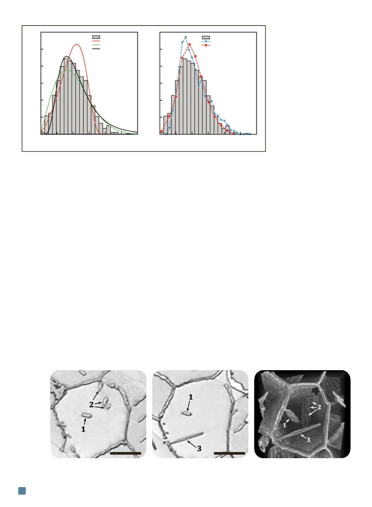
Figure 2 plots the normalized grain size distribution
and shows significant differences between the models and
the experimentally determined distribution of equivalent
sphere radii
[4]
. While the log-normal distribution fits the
peak of the distribution well, it underestimates the number
of small grains and significantly overestimates the number
of large ones. Because a material’s mechanical behavior re-
lies more heavily on the smaller and larger tails of the grain
size distribution, such variations are not acceptable.
Further discrepancies exist between this data and the
two grain growth theories developed by Hillert and
Louat. The Hillert distribution predicts a much sharper
distribution, severely underestimating the number of
large grains, while the Louat distribution is much
broader, predicting a much larger population of smaller
grains. Other 3D data sets acquired of the grain struc-
tures in a nickel-base superalloy
[5]
and recrystallized
alpha iron
[6]
demonstrate similar shortcomings of these
models in reproducing the important tails of grain size
distributions. What is unclear
from the small collection of
3D experimental data is
whether grain size distribu-
tion is somewhat common for
all alloy systems, or if there
are significant deviations
from these distributions that
depend on intrinsic proper-
ties (such as interfacial energy
anisotropies) or extrinsic con-
ditions (such as degree of cold
work before recrystallization).
Cementite precipitate
morphology case study
The differences between the
expectations derived from 2D analyses and the reality re-
vealed through 3D analyses become more evident when
dealing with complex shapes, connectivities, and
nonuniform distributions. This was demonstrated in an
early 3D study by Kral and Spanos
[7]
. Analysis of cemen-
tite morphologies that were visible on 2D section sur-
faces was performed and is shown in Fig. 3a-b. From this,
it was concluded that cementite precipitates form in a
variety of morphologies, with the prevalent morpholo-
gies being grain boundary allotriomorphs (which im-
pinge to form grain boundary films), Widmanstatten
sideplates, intragranular Widmanstatten precipitates,
and intragranular idiomorphs.
Grain boundary allotriomorphs are oblong precipi-
tates, generally viewed as two abutting spherical caps, lo-
cated at the grain boundary that grow to impinge each
other and form a continuous film along the grain bound-
ary as precipitation progresses. Widmanstatten sideplates
are elongated precipitates that nucleate at the grain bound-
ary and extend into the matrix. Elongated precipitates that
lie wholly within the grain are called intragranular Wid-
manstatten plates. Idiomorphs are equiaxed precipitates
typically located within the matrix grain, but occasionally
located at the grain boundary.
Figure 3c shows the actual 3D microstructure of this
alloy, which was revealed through serial sectioning and
ADVANCED MATERIALS & PROCESSES •
SEPTEMBER 2014
18
Fig. 2
—
Comparisons between the equivalent sphere radius grain sizes obtained from
b
-titanium
3D reconstruction and grain size distributions predicted by common models (left) and measured
in other alloys (right).
Fig. 3
—
Optical micrographs of cementite precipitation in an austenite grain, showing different morphologies and connectivities to
the grain boundary of the cementite precipitates (a, b), and 3D reconstruction of that grain demonstrating that all intragranular
precipitates have the same morphology and connectivity (c).
(a)
(b)
(c)
10
m
m
10
m
m
0 0.5 1.0 1.5 2.0 2.5 3.0
R/<R>
0 0.5 1.0 1.5 2.0 2.5 3.0
R/<R>
Ti-21S
b
grains
Ni grains (Groeber 2008)
Fe grains (Zhang 2004)
Ti-21S
b
grains
Hillert (1965)
Louat (1974)
Log normal
1.2
1.0
0.8
0.6
0.4
0.2
0
1.2
1.0
0.8
0.6
0.4
0.2
0
Frequency
Frequency