


 22 / 86

A D V A N C E D M A T E R I A L S & P R O C E S S E S | A P R I L 2 0 1 6
2 2
at room temperature in either uniaxial
compression or using a double-shear
test fixture to approximately 5-8% engi-
neering strain.
SEM data were acquired using a
Carl Zeiss Sigma-VP FEG-SEM. Channel-
ing contrast images were taken at 10 kV
and 0° specimen tilt with a solid-state
backscattered electron detector, yield-
ing both channeling and atomic num-
ber contrast for visualization of slip
lines and
α
/
β
phase distribution. Sub-
sequently, EBSD maps were acquired
at 20 kV accelerating voltage and 70°
specimen tilt using an Oxford Instru-
ments NordlysNano EBSD detector.
During EBSD mapping, secondary elec-
tron and forward-scattered electron
detectors captured images of the EBSD
scan areas. Images and EBSD data were
collected from two locations for each
sample at a magnification sufficient to
examine approximately 50 grains.
After acquiring EBSD scans for
slip-trace analysis, the ATI 6-4 (condi-
tion 4) specimen was re-polished and
rescanned, saving EBSPs at 1344 x
1044 pixels for subsequent processing
with CrossCourt software (BLG Vantage
Software).
POST-ACQUISITION
DATA ANALYSIS
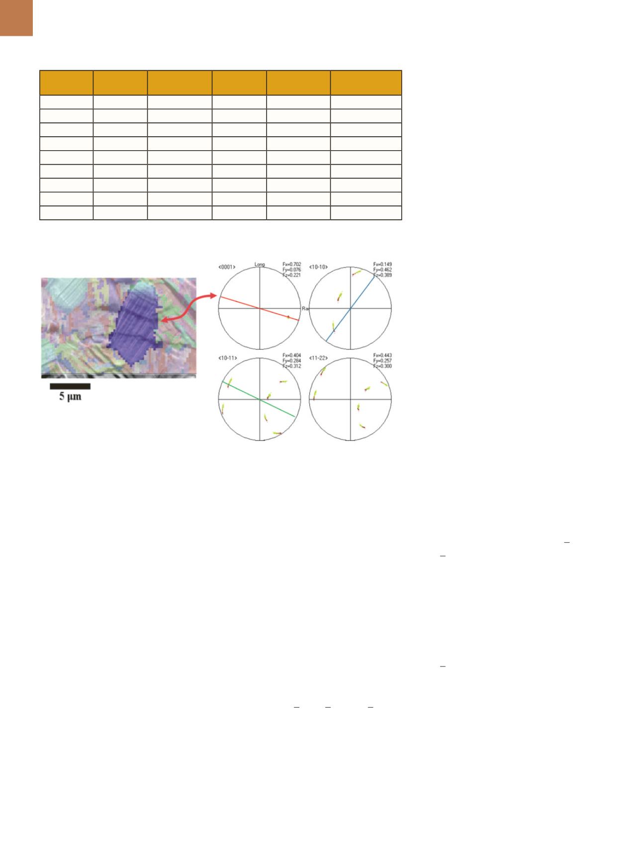
EBSD data from slip band analy-
sis was correlated with images using a
method described by T.R. Bieler, et al.
[2]
.
The trace of the slip line produced on
the polished surface was graphed onto
the {0002}, {1010}, {1011}, or {1122} pole
figures for the specific grain, and visu-
ally matched to intersections with the
plane normal, the intersection of which
identifies the slip system (basal, prism,
1st pyramidal, and 2nd pyramidal, re-
spectively) responsible for the defor-
mation. Between the two EBSD scans
per sample, 20 grains were analyzed for
each material and condition (Fig. 1).
In the HR-EBSD technique used
by CrossCourt 3 software
[3,4]
, the EBSP
of each pixel in a grain is compared
with a reference EBSP via two types of
cross-correlation analysis; one mea-
sures the unit cell distortion, and there-
fore, elastic strain at each pixel; and one
measures whole-body rotations, and,
therefore, plastic strains. The strains
are mapped onto the possible slip sys-
tems in the analyzed material
[4-6]
using
the configuration that yields the min-
imum dislocation line energy
[7]
. This
yields the lower bound of the geomet-
rically necessary dislocations (GND) re-
quired to produce the observed misori-
entation, with a detection threshold as
low as 10
12
lines/m
2
.
RESULTS
Multiple slip bands from each
family of slip systems were observed
in nearly all grains, conditions, and al-
loys. The frequency of each slip system
within a given material and condition
is shown in Table 2. Basal slip occurred
infrequently among all samples, and
loading orientation appeared inconse-
quential when comparing samples 2, 3,
and 4. Conversely, activation of prism
slip bands was significantly different be-
tween samples 2, 3, and 4, demonstrat-
ing that prism slip activation is texture
dependent based on the texture shown
in Fig. 2. It also appeared that {1010} and
{1011} slip bands formedmore frequent-
ly in annealed microstructures.
Figure 3 shows the results of recon-
structing dislocation content using HR-
EBSD analysis. Relevant Burgers vector
and line direction components were cal-
culated using the CrossCourt software
for each slip system, indicating that the
[1120] dislocations of both edge and
screw character were in greater number
density than other directions. However,
no maps show clear signs of slip band
formation, suggesting a difference in
activation energy or interaction of slip
bands within the bulk of the specimens.
DISCUSSION
The HR-EBSD technique is a good
fit for analyzing dislocations in bulk
TABLE 1
—
TEST MATERIALS AND CONDITIONS
Sample
number Material
Max. O
2
content, %
Product
form Condition Loading
direction
1
ATI 6-4
0.20
Wire
Q + A (a)
Longitudinal
2
ATI 6-4
0.20
Wire Annealed (b)
Longitudinal
3
ATI 6-4
0.20
Wire
Annealed
Radial
4
ATI 6-4
0.20
Wire
Annealed Double shear
5
ATI 6-4 ELI
0.13
Wire
Annealed Longitudinal
6
ATI 3-2.5
0.12
Wire
Q + A
Longitudinal
7
ATI 3-2.5
0.12
Wire
Annealed Longitudinal
8
ATI 425
0.30
Wire
Q + A
Longitudinal
9
ATI 425
0.30
Plate
Annealed Longitudinal
(a) Q+A =
α
/
β
solution treated, quenched, and aged. (b)
α
+
β
annealed structure.
Fig. 1 —
Slip line traces translated from the forward-scattered electron image onto the crystallo-
graphic pole figures of the purple grain (red arrow). Each colored line corresponds to a family of
slip lines in the image and with a single family of crystals.