April_AMP_Digital

31 / 50

ADVANCED MATERIALS & PROCESSES • APRIL 2014 31
ters: Rotation speed 850 rpm, travel speed 3.39 mm/s, and
load 15.569 kN. Abaqus software was used as a solver in
the thermal analysis. Temperature-dependent material
properties, density, thermal conductivity, and specific heat
for HSLA-65 were also input to the thermal model. Ther-
mal analysis results were compared with results collected
by Failla and Lippold[1, 2] to verify the thermal model.
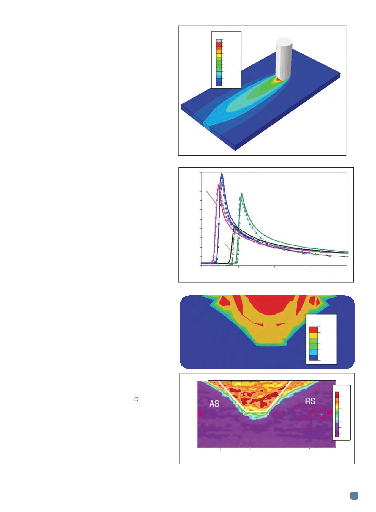
Figure 2 shows the predicted temperature distribution
at 75 seconds. The tool predicts high temperature, but after
the tool moves away, temperature in the weldment cools
down. Figure 3 shows the predicted temperature historic
comparison between the model and experimental measure-
ment[1, 2]. Both model predictions and measurements indi-
cate that the temperature in the FSW stir zone of steel can
be higher than 1200°C. The comparison shows the model
can predict the same temperature distribution observed
during the experiment, thus validating the thermal model.
Microstructure analysis
The predicted temperature evolution was input to the
microstructure model to predict microstructure and hard-
ness. Figure 4 shows a comparison of hardness between
model prediction (Fig. 4a) and experiment[1, 2] (Fig. 4b) at a
weld cross-section. The model predicted hardness in the
tool stir zone close to the hardness measurement. But the
size and shape of the hardness map exhibit some differ-
ences between the prediction and experiment. This may
have occurred due to the difference between FSW tool di-
mensions in the model versus the experiment. Tool dimen-
sions in the model are found by scaling the FSW tool photo
in Ref. 1.
Conclusion
An ICME framework for developing a product using
manufacturing processes includes product requirements,
manufacturing process modeling tools, and the final prod-
uct. Using FSWas an example, model tool development was
introduced, which includes a thermal model, microstruc-
ture model, and mechanical model. The thermal and mi-
crostructure models were validated with experimental data.
Models are able to reasonably predict temperature and hard-
ness distributions as seen in the experiment.
For more information: Yu-Ping Yang is a principal engineer
in the modeling group at EWI, 1250 Arthur E. Adams Dr.,
Columbus, Ohio, 43221, 614/688-5253; ,
References:
1. D.M. Failla, Friction Stir Welding and Microstructure Sim-
ulation of HSLA 65 and Austenitic Stainless Steels, MS The-
sis, The Ohio State University, 2009.
2. D.M. Failla and J. Lippold, Ferrous Alloy Friction Stir Weld-
ing and Microstructure Simulation, FABTECH International
& AWS Welding Show, 2009.
Fig. 4 — Hardness comparison at weld cross-section between prediction
and measurement. (a) Predicted hardness distribution, (b) Measured
hardness map by Failla and Lippold[1, 2].
VHN
320
300
280
260
240
220
200
5 10 15 20×103
Position, µm
10×103
8
6
4
2
Position, µm
HSLA 65 – Weld 431
Hardness
320
300
280
260
240
220
200
(a)
(b)
Fig. 3 — Temperature history comparison of prediction and experiment [1, 2].
Fig. 2 — Predicted temperature evolution during FSW.
Tool
Time = 75 s
Temperature, °C
1289
1200
1100
1000
900
800
700
600
500
400
300
200
100
0
Line-prediction
Symbol-measurement
Weld 431: 850 rpm,
8 imp, 3500 lbf
TC2
TC1
TC3
TC4
0 50 100 150 200
Time, s
1000
900
800
700
600
500
400
300
200
100
0
Temperature, °C